Mapping Economic Landscapes: Clustering and Quantifying Macroeconomic Regimes

Understanding macroeconomic cycles is essential for investors, policymakers, and economists. Economic regimes—distinct periods defined by specific macroeconomic conditions—serve as a critical framework for interpreting these cycles. In this article, we will look how to identify and segregate economic regimes using advanced statistical techniques, highlighting how this approach can provide valuable insights into asset performance and economic forecasting. Drawing on over six decades of data, we apply the Gaussian Mixture Model (GMM) to identify and analyze distinct economic regimes, revealing patterns that can inform dynamic portfolio allocation and policy decisions.

The Concept of Economic Regimes

Economic regimes are characterized by prevailing macroeconomic conditions, including GDP growth, inflation rates, and yield curve behavior. By identifying these regimes, we gain insights into historical trends and can better anticipate future economic shifts. For investors and policymakers, understanding the current regime offers crucial context for decision-making, enabling them to navigate the intricate landscape of economic fluctuations and tailor their strategies accordingly. Recognizing whether the economy is in a period of robust growth, recession, high inflation, or low interest rates helps in making informed decisions that account for current and anticipated economic conditions.

Historical Context and Economic Analysis

The idea of economic regimes is not new. Ray Dalio’s "economic machine" concept suggests that economies move through predictable cycles driven by debt accumulation and deleveraging. Traditional approaches to identifying these cycles often rely on qualitative analysis, which can be subjective. In contrast, our approach uses quantitative techniques to classify regimes, offering a more objective and statistically robust method.

Methodology: Gaussian Mixture Model (GMM) for Regime Classification

Data Sources

To ensure the robustness of our analysis, we compiled macroeconomic data from reputable sources, including the Federal Reserve Economic Data (FRED), the World Bank, and the International Monetary Fund (IMF). The dataset spans from 1970 to 2023 and includes key indicators such as GDP growth, inflation rates, bond yields, and stock market volatility. These variables were selected based on their historical significance in reflecting economic conditions.

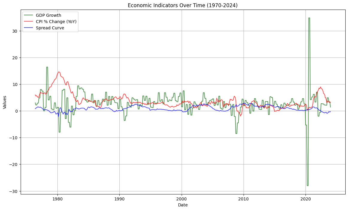
For the purposes of our analysis, I carefully selected three key macroeconomic indicators—GDP growth, CPI inflation, and the yield curve spread (the spread between 10-year and 2-year bond yields)—as inputs to the Gaussian Mixture Model (GMM) for identifying distinct economic regimes. These indicators were chosen based on their historical significance and predictive power in capturing the underlying conditions of different economic periods.

GDP Growth

GDP growth serves as a fundamental measure of economic activity, reflecting the overall health of an economy. It captures the rate at which an economy is expanding or contracting over time. Positive GDP growth indicates economic expansion, while negative growth signifies a contraction, often associated with recessions. By including GDP growth in our GMM, we are able to distinguish between periods of economic prosperity, stagnation, and decline, which are essential for identifying growth, recession, crisis, and recovery regimes.

CPI Inflation

CPI inflation is a critical indicator of price stability and purchasing power within an economy. It measures the rate at which the general price level of goods and services rises, indicating inflationary or deflationary pressures. High inflation can erode consumer purchasing power and signal economic overheating, while low or negative inflation can indicate weak demand and economic distress. By incorporating CPI inflation into our model, we capture the inflationary environment of different regimes, which is crucial for understanding periods of economic stability, hyperinflation, or deflationary spirals.

Yield Curve Spread (10-Year vs. 2-Year Bond Yields)

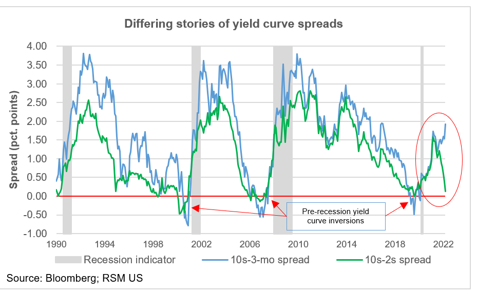
The yield curve spread, specifically the difference between the 10-year and 2-year bond yields, is a powerful predictor of future economic activity. A normal, upward-sloping yield curve suggests investor confidence in future economic growth, as long-term rates are higher than short-term rates. However, an inverted yield curve, where short-term rates exceed long-term rates, is a well-established precursor to economic recessions. Since the 1960s, yield curve inversions have reliably predicted upcoming recessions, making it a critical indicator for our analysis. By including the yield curve spread in our GMM, we can effectively identify and differentiate between regimes associated with economic expansion, imminent recession, and financial crises.

Together, these indicators enable the GMM to classify periods into distinct regimes, reflecting the complex interplay of economic forces at different points in time. This approach enhances our understanding of macroeconomic cycles and provides a robust framework for regime-dependent analysis and decision-making.

Clustering with GMM

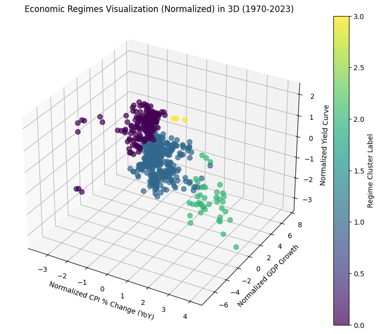
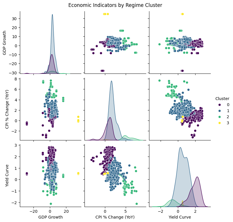
I utilized the Gaussian Mixture Model (GMM) to classify economic regimes. GMM is an unsupervised clustering algorithm that assumes the data is generated from a mixture of several Gaussian distributions, each representing a different economic regime. This model is particularly suitable for our analysis because it allows for the identification of overlapping clusters, which can represent transitional periods between regimes. Below is the 3D visualization of clustering algorithm output across 3 indicators in scope.

Why Gaussian?

The choice of Gaussian distributions is grounded in their flexibility and widespread applicability in representing real-world data. Gaussian distributions are well-suited for capturing the central tendencies and variability of economic indicators, making them ideal for modeling the continuous nature of macroeconomic variables. Additionally, GMM can accommodate the fact that economic data often does not adhere strictly to one regime, instead transitioning smoothly between regimes.

Understanding Four Economic Regimes

Applying the GMM to our dataset we are aiming to distinguish economic regimes: Growth, Recession, Crisis, and Recovery. Each regime is characterized by unique macroeconomic conditions, as detailed in Table 1 below.

Table 1: Economic Regime Characteristics

Regime	GDP Growth	Inflation	Yield Curve	Volatility	Periods
Growth	Moderate	Low	Upward	Low	1982-1989, 1991-2000, 2004-2007, 2010-2019
Recession	Low	High	Inverted	High	1973-1975, 1980-1982, 2001, 2020
Crisis	Negative	Low	Inverted	High	2007-2009, 2020 (COVID-19)
Recovery	High	Moderate	Flattening	Moderate	1983-1991, 2009-2019, 2021-2023

Characterization of Each Regime

Phase 1: Growth

During Growth phases, the economy exhibits robust GDP growth, low inflation, and an upward-sloping yield curve, signaling positive economic expectations. Volatility is subdued, reflecting stability. In these periods, equities and corporate bonds typically perform well, driven by rising investor confidence and economic activity.

Phase 2: Recession

Recession phases are marked by low or negative GDP growth, high inflation, and often a flat or inverted yield curve, indicative of economic pessimism. Volatility increases as markets react to uncertainty. During these periods, safe-haven assets like US Treasurys perform well, while equities and commodities like oil tend to underperform.

Phase 3: Crisis

Crisis phases are characterized by severe economic downturns, with sharply negative GDP growth, low inflation due to diminished economic activity, and an inverted yield curve. Volatility peaks as financial markets experience extreme instability. In these periods, assets like gold and US Treasurys provide safe havens, while equities and oil suffer significant losses.

Phase 4: Recovery

Recovery phases follow crises, with high GDP growth signaling a return to expansion. Inflation moderates, and the yield curve begins to flatten as economic conditions stabilize. Market volatility remains moderate. Equities typically rebound strongly, driven by improved investor sentiment and corporate earnings.

Insights from Regime Classification

Historical Corroboration

The identified regimes correspond closely to well-known historical events, validating the GMM’s ability to detect meaningful economic patterns. For instance, the "Crisis" regime captures periods like the 2008 financial crisis and the COVID-19 pandemic, where economic conditions deteriorated sharply.

Current Economic Environment

As of 2024, the global economy is in Precarious state, resembling conditions observed in early 2007 before the financial crisis. This suggests a period of heightened risk, emphasizing the importance of cautious investment strategies and vigilant economic policy.

Regime-Dependent Asset Performance

Understanding how different asset classes perform across economic regimes is crucial for effective portfolio management. Table 2 below summarizes the average annualized returns for various assets across the four regimes.

Table 2: Asset Class Performance by Economic Regime. Sources: FRED, IMF, World Bank.

Regime	S&P 500 Return	Small Caps Return	US Treasuries Return	Corporate Bonds Return	Gold Return	Oil Return
Growth	8.5%	10.0%	4.0%	3.0%	1.5%	6.0%
Recession	3.2%	-2.0%	10.5%	5.0%	10.5%	15.0%
Crisis	-10.0%	-15.0%	12.0%	8.0%	20.0%	-5.0%
Recovery	10.0%	12.0%	3.5%	4.0%	3.0%	7.0%

Dynamic Portfolio Allocation

Understanding the current economic regime enables dynamic portfolio allocation. During a Growth regime, a portfolio might favor equities and corporate bonds. Conversely, in a Crisis regime, the portfolio might shift towards safer assets like US Treasurys and gold. This regime-dependent strategy allows investors to better navigate economic cycles and optimize returns.

Conclusion

Economic regimes offer a powerful framework for understanding macroeconomic cycles and their impact on asset performance. By leveraging the Gaussian Mixture Model, I demonstrated how to classify these regimes with greater precision, providing valuable insights for investors and policymakers. Although no model can predict the future with absolute certainty, understanding economic regimes equips us with the tools to make informed decisions in a complex global economy. As we continue to refine these models, incorporating new data and methodologies, we can enhance our ability to interpret economic signals and anticipate shifts, ultimately improving decision-making in both investment and policy arenas.